There is strong geological evidence for a single Ice Age, which creation scientists attribute to the aftereffects of the Genesis Flood.¹ However, secular scientists claim that dozens of ice ages have occurred within the last few million years. These ice ages were supposedly paced by subtle variations in the way sunlight falls on the earth, caused by slow changes in Earth’s orbital and rotational motions.

There is strong geological evidence for a single Ice Age, which creation scientists attribute to the aftereffects of the Genesis Flood.

Although this astronomical (or Milankovitch) ice age theory has many problems,² it’s widely accepted because of a well-known 1976 paper titled “Variations in the Earth’s Orbit: Pacemaker of the Ice Ages.”³ This paper examined chemical wiggles called oxygen isotope ratios (denoted by the symbol δ¹⁸O) within two deep-sea sediment cores from the southern Indian Ocean, designated as RC11-120 and E49-18. After assigning timescales to the two cores, the Pacemaker authors found apparent climate cycles with lengths matching the periods of about 100, 41, and 23 thousand years (ka) expected from astronomical calculations, as well as within a composite “PATCH” data set they constructed by combining data segments from the two cores. Thus, the Pacemaker paper was seen as a strong argument for the astronomical ice age theory.

Creation scientists do not accept the vast ages uniformitarian scientists have assigned to these deep-sea cores. However, we will assume those ages for the sake of argument in order to show that secular scientists have since invalidated their own results! This argument, explained in the Part 1 article last month, made use of the fact that the Pacemaker authors assigned time intervals of 273, 363, and 486 ka to their data sets. But the article did not explain how to calculate those time intervals, so here we tie up the loose ends by showing how to do this. Readers who missed Part 1 may wish to read it online at ICR.org.⁴ You may find it helpful to have a copy of the Pacemaker paper to refer to, as well as a copy of a 1973 paper cited by the Pacemaker authors.^3,5

Creation scientists do not accept the vast ages uniformitarian scientists have assigned to these deep-sea cores.

Wiggle Matching and Marine Isotope Stages

Uniformitarian scientists believe that, ideally, the δ¹⁸O record is a global climate indicator. This means that a significant feature, such as a prominent peak or trough, in the δ¹⁸O record within one sediment core should be the same age as a corresponding δ¹⁸O feature within another core. This is thought to be true even if the cores are separated by thousands of miles. So, if ages can somehow be assigned to features within the δ¹⁸O record of one sediment core, those ages can presumably be transferred to the corresponding δ¹⁸O features within other cores—even if they were sourced from halfway around the globe.

In order to facilitate this “wiggle matching” process, uniformitarian scientists devised a numbering system called marine isotope stages (MIS). Numbers are assigned to different parts of the wiggly δ¹⁸O signal. The boundaries between stages are called MIS boundaries.

An Ice Age “Rosetta Stone”

Because radioisotope dating methods generally cannot be used to date seafloor sediments, the Pacemaker authors needed another way to assign ages to the RC11-120 and E49-18 cores. For this, they used another deep-sea core from the western Pacific Ocean, designated as V28-238.

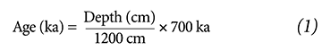
Because seafloor sediments contain magnetic minerals, “flips” or reversals of Earth’s magnetic field can sometimes be identified within the sediments. The most recent of these magnetic reversals is called the Brunhes-Matuyama (B-M) magnetic reversal. Within the V28-238 core, the B-M magnetic reversal was identified at a depth of 1200 centimeters. Secular scientists had already used radioisotope dating to assign an age of 700,000 years (700 ka) to volcanic rocks containing the B-M reversal. Therefore, the sediments at 1200 cm in the V28-238 core were assumed to also be 700 ka. Because the sediments at this location were thought to have been deposited at a nearly constant rate,⁶ and since the age at the top of the V28-238 core was thought to be zero, secular scientists reasoned that sediment age at any given depth in the core could be obtained using this formula:

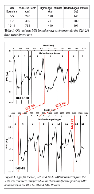
The Pacemaker authors used Equation (1) to assign ages to the MIS boundaries within the V28-238 core—three of which are shown in Table 1. You can verify these ages by substituting the depths from Table 1’s second column into Equation (1). This yields the ages in the table’s third column, which also appear in Table 3 of the 1973 paper.⁵ Believing the δ¹⁸O signal to be a global climate indicator, the Pacemaker authors transferred these three ages to the presumed corresponding MIS boundaries within the RC11-120 and E49-18 cores (Figure 1).^3,5,7 They then used these ages to set up the timescales for those two cores.

Age Models

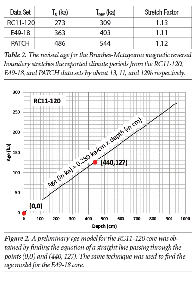
The Pacemaker authors first assigned simple age models (which they called SIMPLEX) to the RC11-120 and E49-18 cores. They assumed the sediments within a core were deposited at a constant rate and used the ages at two different depths to find that rate. These depths and their corresponding ages are listed at the top of their Table 2. For the RC11-120 core (see Figure 2), they used the core top (depth of 0 cm) and the MIS 6-5 boundary (depth of 440 cm). The age of the top of the RC11-120 core was assumed to be 0 ka, and the age at 440 cm depth was assumed to be 127 ka.^3,7 So, the Pacemaker authors found the equation of a straight line passing through the points (0, 0) and (440, 127) to obtain a formula that assigned ages to different depths within the RC11-120 core:

age_RC11-120 (in ka)=0.289ka/cm × depth (in cm) (2)

Even if your high school algebra is rusty, you can still check that Equation (2) is correct. Substituting a depth of 0 cm into Equation (2) yields an age of 0 ka, as required, and a depth of 440 cm yields an age of 127 ka, also as required.

The Pacemaker authors used the same procedure to assign ages to the bottom section of the E49-18 core; they only used depths at or below 490 cm in their analysis.³ They used the 6-5 and 12-11 MIS boundaries in the E49-18 core, located at depths of 490 and 1405 cm respectively, to calculate the equation of a straight line passing through the points (490, 127) and (1405, 440):

age_{bottom of E49-18} (in ka)=0.342ka/cm × depth (in cm) – 40.619 ka (3)

Again, substituting depths of 490 cm and 1405 cm into Equation (3) yields respective ages of 127 ka and 440 ka, as required.

Calculating the Original Time Intervals

According to Table 3 of the Pacemaker paper, the total time interval assigned to the RC11-120 core was 273 ka. How was this number obtained? The RC11-120 core was 950 cm long, so inserting a depth of 950 cm into Equation (2) gives the presumed age at the core bottom: 0.289 ka/cm × 950 cm = 275 ka. However, one of the “quirks” of the method of spectral analysis used by the Pacemaker authors is that the data points used in the analysis must be separated by precisely equal time intervals.⁸ Even for the simple age models in Equations (2) and (3), round-off errors usually cause slight differences in the time intervals between data points. So, one usually has to replace the original data set with an “interpolated” data set that mimics the original data set but whose data points are spaced perfectly evenly in time. Because the Pacemaker authors chose a time interval of 3,000 years (3 ka) to separate their interpolated data points,³ the total time interval assigned to the RC11-120 core had to be an integer multiple of 3 ka. The highest number less than 275 ka that meets this requirement is 273 ka, as shown in their Table 3.

Likewise, the 1550 cm length of the E49-18 core was used to find the total time interval assigned to the bottom section of the E49-18 core. Inserting 1550 cm and 490 cm into Equation (3) yields respective ages of 489 ka and 127 ka (see their Table 3). Subtracting these two numbers and rounding to the nearest integer multiple of 3 ka gives a time interval of 363 ka.

After obtaining initial results favorable to the astronomical theory, they applied a more complicated ELBOW age model to the PATCH data set that used four straight-line segments instead of just one. Although I don’t show the math here due to space constraints, you can use algebra and the ELBOW data in their Table 2 to verify that this resulted in a total time interval of 486 ka for the PATCH data set.^9,10

New Timescales

However, in the early 1990s, secular scientists changed the age claimed for the B-M magnetic reversal boundary to 780 ka.⁶ So, by their own reckoning, the ages they originally assigned to the MIS boundaries are no longer valid. And since the Pacemaker results depended on these ages, the Pacemaker results are invalid, too! You can confirm the revised MIS boundary age estimates (fourth column of Table 1) by changing the 700 in Equation (1) to 780 and re-doing the calculations. The same procedure as before yields new SIMPLEX age equations for the two cores:

age_RC11-120 (in ka)=0.325ka/cm × depth (in cm) (4)

age_{bottom of E49-18} (in ka)=0.380ka/cm × depth (in cm) – 43.227 ka (5)

These equations yield new time intervals of 309 and 403 ka for the RC11-120 and E49-18 cores. The new time interval assigned to the PATCH data set is 544 ka.

Unfortunately for Milankovitch proponents, most of these new climate periods no longer agree with the astronomical expectations!

Conclusion

Now that you know how the ages were assigned to the Indian Ocean cores, you can verify the results presented in last month’s Part 1 article. The new age assignment for the B-M magnetic reversal boundary stretches the climate periods originally reported in Tables 3 and 4 of the Pacemaker paper. Some reflection shows that the method described in Part 1 is equivalent to dividing the new time interval T_new for a core by the original time interval T₀ to calculate a “core stretch factor” (my Table 2). Multiplying the stretch factor for a particular data set by the climate periods reported for that data set (in their Tables 3 and 4) gives the new climate periods. Unfortunately for Milankovitch proponents, most of these new climate periods no longer agree with the astronomical expectations!⁴

Without the Pacemaker results, it is doubtful there’s any convincing evidence for the Milankovitch theory, even by secular reckoning. Yet, many scientists routinely use the astronomical theory as an age-dating method, and the theory is making subtle contributions to global warming alarmism.¹¹ Secular scientists are either unaware of this age revision and its implications or they’re ignoring them. How, then, can anyone trust these scientists’ pronouncements about Earth history and climate change if they have allowed this error in such an important paper to go uncorrected for over 25 years?

Click here to read “Testing Old-Earth Climate Claims, Part 1.”

References

1. Hebert, J. 2013. Was There An Ice Age? Acts & Facts. 42 (12): 20.
2. Oard, M. J. 2007. Astronomical troubles for the astronomical hypothesis of ice ages. Journal of Creation. 21 (3): 19-23.
3. Hays, J. D., J. Imbrie, and N. J. Shackleton. 1976. Variations in the Earth’s Orbit: Pacemaker of the Ice Ages. Science. 194 (4270): 1121-1132.
4. Hebert, J. 2017. Testing Old-Earth Climate Claims, Part 1. Acts & Facts. 46 (11): 10-13.
5. Shackleton, N. J. and N. D. Opdyke.1973. Oxygen Isotope and Palaeomagnetic Stratigraphy of Equatorial Pacific Core V28-238: Oxygen Isotope Temperatures and Ice Volumes on a 105 Year and 106 Year Scale. Quaternary Research. 3 (1): 39-55. Copies of this paper (reference 31 in the Pacemaker paper) may be purchased at cambridge.org.
6. Shackleton, N. J., A. Berger, and W. R. Peltier. 1990. An Alternative Astronomical Calibration of the Lower Pleistocene Timescale Based on ODP Site 677. Transactions of the Royal Society of Edinburgh: Earth Sciences. 81 (4): 251-261.
7. The Pacemaker authors felt the age of 127 ka, obtained by other means, was slightly more accurate than the age of 128 ka.
8. Blackman, R. B. and J. W. Tukey. 1958. The Measurement of Power Spectra from the Point of View of Communications Engineering. New York: Dover Publications.
9. The Pacemaker paper erroneously reports this time as 468 ka in the caption to their Table 4, but the authors transposed the 6 and the 8 (468 is not evenly divisible by 3, but 486 ka is).
10. The Pacemaker authors’ “Tune-Up” age model is only justified if the results from the SIMPLEX and ELBOW age models were in good agreement with the astronomical theory.
11. Hebert, J. 2017. Milankovitch Meltdown: Toppling an Iconic Old-Earth Argument, Part 3. Acts & Facts. 46 (1): 10-13.

* Dr. Hebert is Research Associate at the Institute for Creation Research and earned his Ph.D. in physics from the University of Texas at Dallas.